
Packed Selection#
This is a rendered copy of packedselection.ipynb. You can optionally run it interactively on binder at this link
In coffea, PackedSelection is a class that can store several boolean arrays in a memory-efficient manner and evaluate arbitrary combinations of boolean requirements in an CPU-efficient way. Supported inputs include 1D numpy or awkward arrays and it has built-in functionalities to form analysis in signal and control regions, and to implement cutflow or “N-1” plots.
coffea 2025 supports multiple modes, including eager (which loads all data from the file, typically best for testing only small input files), virtual (which functions the most like coffea 0.7 and only loads data as-needed), and dask (the original variation introduced in CalVer coffea to utilize fully DAG-building via dask / dask-awkward). Let’s first read a sample file of 40 Drell-Yan events to demonstrate the utilities using our NanoAODSchema as our schema; feel free to swap between eager and virtual modes for the events array.
import awkward as ak
import numpy as np
from coffea.nanoevents import NanoEventsFactory, NanoAODSchema
from matplotlib import pyplot as plt

NanoAODSchema.warn_missing_crossrefs = False

fname = "coffea/tests/samples/nano_dy.root"
events = NanoEventsFactory.from_root(
    {fname: "Events"},
    metadata={"dataset": "nano_dy"},
    schemaclass=NanoAODSchema,
    mode="eager",
).events()

events
[{Electron: [], PuppiMET: {phi: 1.64, ...}, FsrPhoton: [], ChsMET: {...}, ...},
 {Electron: [{deltaEtaSC: -0.0145, ...}], PuppiMET: {...}, FsrPhoton: [], ...},
 {Electron: [Electron, ...], PuppiMET: {...}, ...},
 {Electron: [Electron, ...], PuppiMET: {...}, ...},
 {Electron: [], PuppiMET: {phi: 0.538, ...}, FsrPhoton: [], ChsMET: {...}, ...},
 {Electron: [{deltaEtaSC: -0.0232, ...}], PuppiMET: {...}, FsrPhoton: [], ...},
 {Electron: [{deltaEtaSC: 0.00415, ...}], PuppiMET: {...}, FsrPhoton: [], ...},
 {Electron: [], PuppiMET: {phi: 0.105, ...}, FsrPhoton: [], ChsMET: {...}, ...},
 {Electron: [], PuppiMET: {phi: -0.513, ...}, FsrPhoton: [], ChsMET: ..., ...},
 {Electron: [{deltaEtaSC: 0.00813, ...}], PuppiMET: {...}, FsrPhoton: [], ...},
 ...,
 {Electron: [{deltaEtaSC: -0.00836, ...}], PuppiMET: {...}, ...},
 {Electron: [], PuppiMET: {phi: 0.612, ...}, FsrPhoton: [], ChsMET: {...}, ...},
 {Electron: [{deltaEtaSC: -0.00405, ...}], PuppiMET: {...}, ...},
 {Electron: [], PuppiMET: {phi: 2.83, ...}, FsrPhoton: [], ChsMET: {...}, ...},
 {Electron: [{deltaEtaSC: 0.053, ...}], PuppiMET: {...}, FsrPhoton: [], ...},
 {Electron: [], PuppiMET: {phi: 1.44, ...}, FsrPhoton: [], ChsMET: {...}, ...},
 {Electron: [{deltaEtaSC: -0.00986, ...}], PuppiMET: {...}, ...},
 {Electron: [], PuppiMET: {phi: -2.92, ...}, FsrPhoton: [], ChsMET: {...}, ...},
 {Electron: [], PuppiMET: {phi: -0.415, ...}, FsrPhoton: [], ChsMET: ..., ...}]
--------------------------------------------------------------------------------
backend: cpu
nbytes: 243.3 kB
type: 40 * event
Now let’s import PackedSelection, and create an instance of it.
from coffea.analysis_tools import PackedSelection

selection = PackedSelection()
We can create a boolean mask and add this to our selection by using the add method. This adds the following “cut” to our selection and names it “twoElectron”.
selection.add("twoElectron", ak.num(events.Electron) == 2)
We’ve added one “cut” to our selection. Now let’s add a couple more.
selection.add("eleOppSign", ak.sum(events.Electron.charge, axis=1) == 0)
selection.add("noElectron", ak.num(events.Electron) == 0)
To avoid repeating calling add multiple times, we can just use the add_multiple method which does just that.
selection.add_multiple(
    {
        "twoMuon": ak.num(events.Muon) == 2,
        "muOppSign": ak.sum(events.Muon.charge, axis=1) == 0,
        "noMuon": ak.num(events.Muon) == 0,
        "leadPt20": ak.any(events.Electron.pt >= 20.0, axis=1) | ak.any(events.Muon.pt >= 20.0, axis=1),
    }
)
By viewing the PackedSelection instance, one can see the names of the added selections, whether it is operating in delayed mode or not, the number of added selections and the maximum supported number of selections.
print(selection)
PackedSelection(selections=('twoElectron', 'eleOppSign', 'noElectron', 'twoMuon', 'muOppSign', 'noMuon', 'leadPt20'), delayed_mode=False, items=7, maxitems=32)
To evaluate a boolean mask (e.g. to filter events) we can use the selection.all(*names) function, which will compute the logical AND of all listed boolean selections.
selection.all("twoElectron", "noMuon", "leadPt20")
array([False, False,  True, False, False, False, False, False, False,
       False, False, False, False, False, False, False, False, False,
       False, False,  True,  True, False, False, False, False, False,
       False, False, False, False, False, False, False, False, False,
       False, False, False, False])
We can also be more specific and require that a specific set of selections have a given value (with the unspecified ones allowed to be either true or false) using selection.require.
selection.require(twoElectron=True, noMuon=True, eleOppSign=False)
array([False, False, False,  True, False, False, False, False, False,
       False, False, False, False, False, False, False, False, False,
       False, False, False, False, False, False, False, False, False,
       False, False, False, False, False, False, False, False, False,
       False, False, False, False])
There exist also the allfalse and any methods where the first one is the opposite of all and the second one is a logical OR between all listed boolean selections.
Using PackedSelection, we are now able to perform an N-1 style selection using the nminusone(*names) method. This will perform an N-1 style selection by using as “N” the provided names and will exclude each named cut one at a time in order. In the end it will also peform a selection using all N cuts.
nminusone = selection.nminusone("twoElectron", "noMuon", "leadPt20")
nminusone
NminusOne(selections=('twoElectron', 'noMuon', 'leadPt20'), commonmasked=False, weighted=False, weightsmodifier=None)
This returns an NminusOne object which has the following methods: result(), print(), yieldhist(), to_npz() and plot_vars()
Let’s look at the results of the N-1 selection.
res = nminusone.result()
print(type(res), res._fields)
<class 'coffea.analysis_tools.NminusOneResult'> ('labels', 'nev', 'masks')
This is just a namedtuple with the attributes labels, nev and masks. So we can say:
labels, nev, masks = res
labels, nev, masks
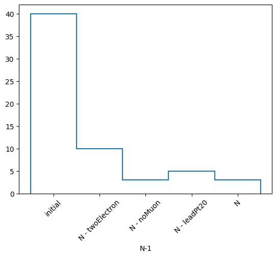
(['initial', 'N - twoElectron', 'N - noMuon', 'N - leadPt20', 'N'],
 [40, np.int64(10), np.int64(3), np.int64(5), np.int64(3)],
 [array([False,  True,  True, False, False, False, False, False, False,
          True, False, False, False, False, False,  True,  True, False,
         False, False,  True,  True, False, False, False, False, False,
          True, False,  True, False, False, False,  True, False, False,
         False, False, False, False]),
  array([False, False,  True, False, False, False, False, False, False,
         False, False, False, False, False, False, False, False, False,
         False, False,  True,  True, False, False, False, False, False,
         False, False, False, False, False, False, False, False, False,
         False, False, False, False]),
  array([False, False,  True,  True, False, False, False, False, False,
         False, False, False, False, False, False, False, False, False,
          True, False,  True,  True, False, False, False, False, False,
         False, False, False, False, False, False, False, False, False,
         False, False, False, False]),
  array([False, False,  True, False, False, False, False, False, False,
         False, False, False, False, False, False, False, False, False,
         False, False,  True,  True, False, False, False, False, False,
         False, False, False, False, False, False, False, False, False,
         False, False, False, False])])
labels is a list of labels of each mask that is applied, nev is a list of the number of events that survive each mask, and masks is a list of boolean masks (arrays) of which events survive each selection.
You can also choose to print the statistics of your N-1 selection in a similar fashion to RDataFrame.
nminusone.print()
N-1 selection stats:
Ignoring twoElectron pass = 10 all = 40 -- eff = 25.0 %
Ignoring noMuon pass = 3 all = 40 -- eff = 7.5 %
Ignoring leadPt20 pass = 5 all = 40 -- eff = 12.5 %
All cuts pass = 3 all = 40 -- eff = 7.5 %
Or get a histogram of your total event yields. This just returns a hist.Hist object and we can plot it with its backends to mplhep.
h, labels = nminusone.yieldhist()
h.plot1d()
plt.xticks(plt.gca().get_xticks(), labels, rotation=45)
plt.show()
You can also save the results of the N-1 selection to a .npz file for later use.
nminusone.to_npz("nminusone_results.npz").compute()
with np.load("nminusone_results.npz") as f:
    for i in f.files:
        print(f"{i}: {f[i]}")
labels: ['initial' 'N - twoElectron' 'N - noMuon' 'N - leadPt20' 'N']
nev: [40 10  3  5  3]
masks: [[False  True  True False False False False False False  True False False
  False False False  True  True False False False  True  True False False
  False False False  True False  True False False False  True False False
  False False False False]
 [False False  True False False False False False False False False False
  False False False False False False False False  True  True False False
  False False False False False False False False False False False False
  False False False False]
 [False False  True  True False False False False False False False False
  False False False False False False  True False  True  True False False
  False False False False False False False False False False False False
  False False False False]
 [False False  True False False False False False False False False False
  False False False False False False False False  True  True False False
  False False False False False False False False False False False False
  False False False False]]
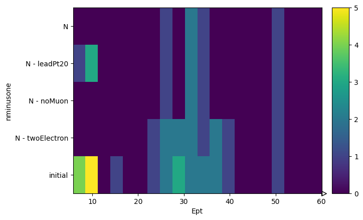
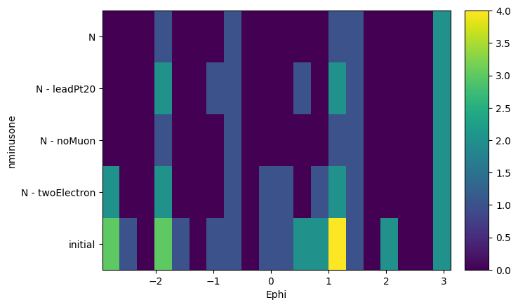
Finally, we can ask from this object to create histograms of different variables, masking them with our N-1 selection. What it will output is a list of histograms, one for each requested variable, where the x-axis is the distribution of the variable, and the y-axis is the mask that was applied. It is essentially slices of how the variable distribution evolves as each N-1 or N selection is applied. It does also return a list of labels of the masks to keep track.
Note that the variables are parsed using a dictonary of name: array pairs and that the arrays will of course be flattened to be histogrammed.
hs, labels = nminusone.plot_vars({"Ept": events.Electron.pt, "Ephi": events.Electron.phi})
hs, labels
([Hist(
    Regular(20, 5.81891, 60.0685, name='Ept'),
    Integer(0, 5, name='nminusone'),
    storage=Double()) # Sum: 55.0 (60.0 with flow),
  Hist(
    Regular(20, -2.93115, 3.11865, name='Ephi'),
    Integer(0, 5, name='nminusone'),
    storage=Double()) # Sum: 60.0],
 ['initial', 'N - twoElectron', 'N - noMuon', 'N - leadPt20', 'N'])
And we can actually plot those histograms using again the mplhep backend.
for h in hs:
    h.plot2d()
    plt.yticks(plt.gca().get_yticks(), labels, rotation=0)
    plt.show()
You can slice these histograms to view and plot the 1D histogram at each step of the selection. For example, if we want the $P_T$ of the electrons at the final step (index 4) of the selection, we can do the following.
hs[0][:, 4].plot1d(yerr=0)
plt.yscale("log")
plt.show()
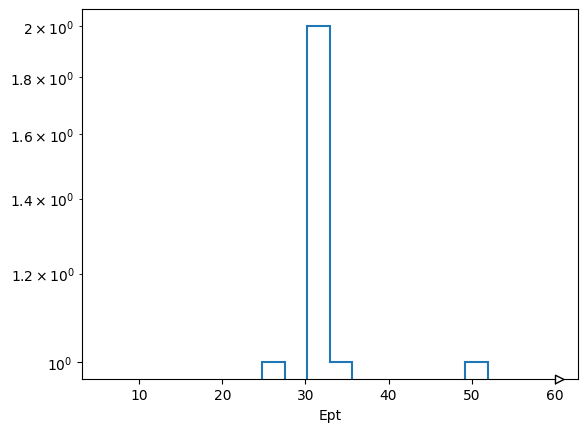
Because this automatic bining doesn’t look great, for $P_T$ at least, the user has the ability to customize the axes or pass in their own axes objects.
help(nminusone.plot_vars)
Help on method plot_vars in module coffea.analysis_tools:

plot_vars(
    vars,
    axes=None,
    bins=None,
    start=None,
    stop=None,
    edges=None,
    transform=None,
    weighted=None,
    scale=None,
    categorical=None
) method of coffea.analysis_tools.NminusOne instance
    Plot the histograms of variables for each step of the N-1 selection

    Parameters
    ----------
        vars : dict
            A dictionary in the form ``{name: array}`` where ``name`` is the name of the variable,
            and ``array`` is the corresponding array of values.
            The arrays must be the same length as each mask of the N-1 selection.
        axes : list of hist.axis objects, optional
            The axes objects to histogram the variables on. This will override all the following arguments that define axes.
            Must be the same length as ``vars``.
        bins : iterable of integers or Nones, optional
            The number of bins for each variable histogram. If not specified, it defaults to 20.
            Must be the same length as ``vars``.
        start : iterable of floats or integers or Nones, optional
            The lower edge of the first bin for each variable histogram. If not specified, it defaults to the minimum value of the variable array.
            Must be the same length as ``vars``.
        stop : iterable of floats or integers or Nones, optional
            The upper edge of the last bin for each variable histogram. If not specified, it defaults to the maximum value of the variable array.
            Must be the same length as ``vars``.
        edges : list of iterables of floats or integers, optional
            The bin edges for each variable histogram. This overrides ``bins``, ``start``, and ``stop`` if specified.
            Must be the same length as ``vars``.
        transform : iterable of hist.axis.transform objects or Nones, optional
            The transforms to apply to each variable histogram axis. If not specified, it defaults to None.
            Must be the same length as ``vars``.
        weighted : bool, optional
            Whether to fill the histograms with weights. Default is None, which applies the weights
            if the nminusone was instantiated with weights and unweighted distributions otherwise.
        scale: float, optional
            A scalar value by which all weights will be scaled, works with both weighted and unweighted methods.
        categorical : dict, optional
            A dictionary with the following keys:
                axis : hist.axis object
                    The axis to be used as a categorical axis
                values : list
                    The array to be filled in the categorical axis, must be the same length as the masks
                labels : list
                    The labels corresponding to the values in the categorical axis
            Default is None, which does not apply any categorical axis.

    Returns
    -------
        hists : list of hist.Hist or hist.dask.Hist objects
            A list of 2D histograms of the variables for each step of the N-1 selection.
            The first axis is the variable, the second axis is the N-1 selection step.
        labels : list of strings
            The bin labels of y axis of the histogram.
        catlabels : list of strings, optional
            The labels of the categorical axis
Cutflow is implemented in a similar manner to the N-1 selection. We just have to use the cutflow(*names) function which will return a Cutflow object
cutflow = selection.cutflow("noMuon", "twoElectron", "leadPt20")
cutflow
Cutflow(selections=('noMuon', 'twoElectron', 'leadPt20'), commonmasked=False, weighted=False, weightsmodifier=None)
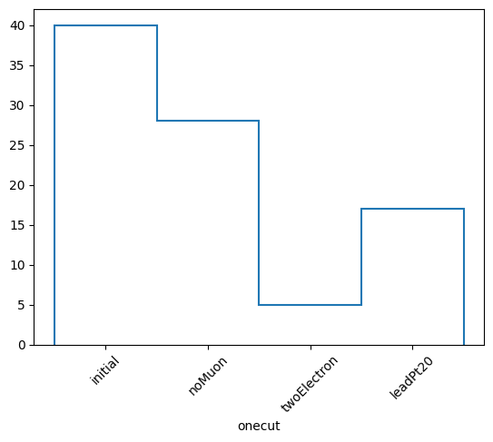
The methods of this object are similar to the NminusOne object. The only difference is that now we seperate things in either “onecut” or “cutflow”. “onecut” represents results where each cut is applied alone, while “cutflow” represents results where the cuts are applied cumulatively in order.
res = cutflow.result()
print(type(res), res._fields)
labels, nevonecut, nevcutflow, masksonecut, maskscutflow = res
labels, nevonecut, nevcutflow, masksonecut, maskscutflow
<class 'coffea.analysis_tools.CutflowResult'> ('labels', 'nevonecut', 'nevcutflow', 'masksonecut', 'maskscutflow')
(['initial', 'noMuon', 'twoElectron', 'leadPt20'],
 [40, np.int64(28), np.int64(5), np.int64(17)],
 [40, np.int64(28), np.int64(5), np.int64(3)],
 [array([ True,  True,  True,  True, False, False, False,  True,  True,
          True, False,  True,  True,  True, False,  True,  True,  True,
          True,  True,  True,  True,  True, False, False,  True, False,
          True, False,  True, False, False,  True,  True, False,  True,
          True,  True,  True,  True]),
  array([False, False,  True,  True, False, False, False, False, False,
         False, False, False, False, False, False, False, False, False,
          True, False,  True,  True, False, False, False, False, False,
         False, False, False, False, False, False, False, False, False,
         False, False, False, False]),
  array([False,  True,  True, False,  True,  True,  True, False, False,
          True, False, False, False, False, False,  True,  True, False,
         False, False,  True,  True, False,  True,  True, False,  True,
          True, False,  True, False,  True, False,  True, False, False,
         False, False, False, False])],
 [array([ True,  True,  True,  True, False, False, False,  True,  True,
          True, False,  True,  True,  True, False,  True,  True,  True,
          True,  True,  True,  True,  True, False, False,  True, False,
          True, False,  True, False, False,  True,  True, False,  True,
          True,  True,  True,  True]),
  array([False, False,  True,  True, False, False, False, False, False,
         False, False, False, False, False, False, False, False, False,
          True, False,  True,  True, False, False, False, False, False,
         False, False, False, False, False, False, False, False, False,
         False, False, False, False]),
  array([False, False,  True, False, False, False, False, False, False,
         False, False, False, False, False, False, False, False, False,
         False, False,  True,  True, False, False, False, False, False,
         False, False, False, False, False, False, False, False, False,
         False, False, False, False])])
As you can see, again we have the same labels, nev and masks only now we have two “versions” of them since they’ve been split into “onecut” and “cutflow”.
You can again print the statistics of the cutflow exactly like RDataFrame.
cutflow.print()
Cutflow selection stats:
Cut noMuon              :pass = 28                  cumulative pass = 28                  all = 40
-- eff = 70.0 %                    -- cumulative eff = 70.0 %
Cut twoElectron         :pass = 5                   cumulative pass = 5                   all = 40
-- eff = 12.5 %                    -- cumulative eff = 12.5 %
Cut leadPt20            :pass = 17                  cumulative pass = 3                   all = 40
-- eff = 42.5 %                    -- cumulative eff = 7.5 %
Again, you can extract yield hists, only now there are two of them.
honecut, hcutflow, labels = cutflow.yieldhist()
honecut.plot1d(yerr=0)
plt.xticks(plt.gca().get_xticks(), labels, rotation=45)
plt.show()
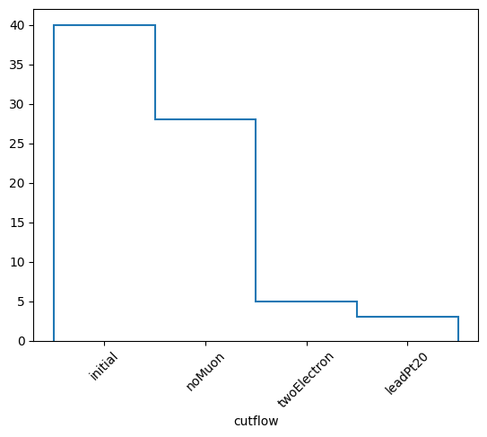
hcutflow.plot1d(yerr=0)
plt.xticks(plt.gca().get_xticks(), labels, rotation=45)
plt.show()
Saving to .npz files is again there.
cutflow.to_npz("cutflow_results.npz").compute()

with np.load("cutflow_results.npz") as f:
    for i in f.files:
        print(f"{i}: {f[i]}")
labels: ['initial' 'noMuon' 'twoElectron' 'leadPt20']
nevonecut: [40 28  5 17]
nevcutflow: [40 28  5  3]
masksonecut: [[ True  True  True  True False False False  True  True  True False  True
   True  True False  True  True  True  True  True  True  True  True False
  False  True False  True False  True False False  True  True False  True
   True  True  True  True]
 [False False  True  True False False False False False False False False
  False False False False False False  True False  True  True False False
  False False False False False False False False False False False False
  False False False False]
 [False  True  True False  True  True  True False False  True False False
  False False False  True  True False False False  True  True False  True
   True False  True  True False  True False  True False  True False False
  False False False False]]
maskscutflow: [[ True  True  True  True False False False  True  True  True False  True
   True  True False  True  True  True  True  True  True  True  True False
  False  True False  True False  True False False  True  True False  True
   True  True  True  True]
 [False False  True  True False False False False False False False False
  False False False False False False  True False  True  True False False
  False False False False False False False False False False False False
  False False False False]
 [False False  True False False False False False False False False False
  False False False False False False False False  True  True False False
  False False False False False False False False False False False False
  False False False False]]
And finally, plot_vars is also there with the same axes customizability while now it returns two lists of histograms, one for “onecut” and one for “cutflow”. Those can of course be plotted in a similar fashion.
h1, h2, labels = cutflow.plot_vars({"ept": events.Electron.pt, "ephi": events.Electron.phi})
h1, h2, labels
([Hist(
    Regular(20, 5.81891, 60.0685, name='ept'),
    Integer(0, 4, name='onecut'),
    storage=Double()) # Sum: 69.0 (73.0 with flow),
  Hist(
    Regular(20, -2.93115, 3.11865, name='ephi'),
    Integer(0, 4, name='onecut'),
    storage=Double()) # Sum: 73.0],
 [Hist(
    Regular(20, 5.81891, 60.0685, name='ept'),
    Integer(0, 4, name='cutflow'),
    storage=Double()) # Sum: 59.0 (63.0 with flow),
  Hist(
    Regular(20, -2.93115, 3.11865, name='ephi'),
    Integer(0, 4, name='cutflow'),
    storage=Double()) # Sum: 63.0],
 ['initial', 'noMuon', 'twoElectron', 'leadPt20'])
Weighted Cutflows and NMinusOnes#
It’s also possible to apply per-event weights to a cutflow/nminusone by passing in a Weights instance, along with the weightsmodifier (None or the string name of the variation you want applied)
from coffea.analysis_tools import Weights

weights = Weights(len(events))
weights.add("genweight", events.genWeight)

wgtcutflow = selection.cutflow("noMuon", "twoElectron", "leadPt20", weights=weights, weightsmodifier=None)
wgtcutflow
Cutflow(selections=('noMuon', 'twoElectron', 'leadPt20'), commonmasked=False, weighted=True, weightsmodifier=None)
res = wgtcutflow.result()
print(type(res), res._fields)
(labels, nevonecut, nevcutflow, masksonecut, maskscutflow, commonmask, wgtevonecut, wgtevcutflow, rweights, rmod) = res
labels, nevonecut, nevcutflow, masksonecut, maskscutflow, commonmask, wgtevonecut, wgtevcutflow, rweights, rmod
<class 'coffea.analysis_tools.ExtendedCutflowResult'> ('labels', 'nevonecut', 'nevcutflow', 'masksonecut', 'maskscutflow', 'commonmask', 'wgtevonecut', 'wgtevcutflow', 'weights', 'weightsmodifier')
(['initial', 'noMuon', 'twoElectron', 'leadPt20'],
 [40, np.int64(28), np.int64(5), np.int64(17)],
 [40, np.int64(28), np.int64(5), np.int64(3)],
 [array([ True,  True,  True,  True, False, False, False,  True,  True,
          True, False,  True,  True,  True, False,  True,  True,  True,
          True,  True,  True,  True,  True, False, False,  True, False,
          True, False,  True, False, False,  True,  True, False,  True,
          True,  True,  True,  True]),
  array([False, False,  True,  True, False, False, False, False, False,
         False, False, False, False, False, False, False, False, False,
          True, False,  True,  True, False, False, False, False, False,
         False, False, False, False, False, False, False, False, False,
         False, False, False, False]),
  array([False,  True,  True, False,  True,  True,  True, False, False,
          True, False, False, False, False, False,  True,  True, False,
         False, False,  True,  True, False,  True,  True, False,  True,
          True, False,  True, False,  True, False,  True, False, False,
         False, False, False, False])],
 [array([ True,  True,  True,  True, False, False, False,  True,  True,
          True, False,  True,  True,  True, False,  True,  True,  True,
          True,  True,  True,  True,  True, False, False,  True, False,
          True, False,  True, False, False,  True,  True, False,  True,
          True,  True,  True,  True]),
  array([False, False,  True,  True, False, False, False, False, False,
         False, False, False, False, False, False, False, False, False,
          True, False,  True,  True, False, False, False, False, False,
         False, False, False, False, False, False, False, False, False,
         False, False, False, False]),
  array([False, False,  True, False, False, False, False, False, False,
         False, False, False, False, False, False, False, False, False,
         False, False,  True,  True, False, False, False, False, False,
         False, False, False, False, False, False, False, False, False,
         False, False, False, False])],
 None,
 [np.float64(578762.435546875),
  np.float64(315450.423828125),
  np.float64(25807.2109375),
  np.float64(237244.12109375)],
 [np.float64(578762.435546875),
  np.float64(315450.423828125),
  np.float64(25807.2109375),
  np.float64(26331.201171875)],
 <coffea.analysis_tools.Weights at 0x1425f2cf0>,
 None)
The weighted cutflow by default prints with weights if included, but passing weighted=False or weighted=True allows one to explicitly toggle between the two. Additionally, the keyword scale permits one to scale all value uniformly, such as with a cross-section, luminosity, sum of weights, etc.
wgtcutflow.print()
Cutflow selection stats: (weighted)
Cut noMuon              :pass = 315450.423828125    cumulative pass = 315450.423828125    all = 578762.435546875
-- eff = 54.5 %                    -- cumulative eff = 54.5 %
Cut twoElectron         :pass = 25807.2109375       cumulative pass = 25807.2109375       all = 578762.435546875
-- eff = 4.5 %                    -- cumulative eff = 4.5 %
Cut leadPt20            :pass = 237244.12109375     cumulative pass = 26331.201171875     all = 578762.435546875
-- eff = 41.0 %                    -- cumulative eff = 4.5 %
wgtcutflow.print(weighted=False)
Cutflow selection stats:
Cut noMuon              :pass = 28                  cumulative pass = 28                  all = 40
-- eff = 70.0 %                    -- cumulative eff = 70.0 %
Cut twoElectron         :pass = 5                   cumulative pass = 5                   all = 40
-- eff = 12.5 %                    -- cumulative eff = 12.5 %
Cut leadPt20            :pass = 17                  cumulative pass = 3                   all = 40
-- eff = 42.5 %                    -- cumulative eff = 7.5 %
wgtcutflow.print(weighted=True, scale=500 / 578762)
Cutflow selection stats: (weighted) (scaled by 0.0008639129728627657)
Cut noMuon              :pass = 272.5217134401749   cumulative pass = 272.5217134401749   all = 500.0003762745956
-- eff = 54.5 %                    -- cumulative eff = 54.5 %
Cut twoElectron         :pass = 22.295184322312107  cumulative pass = 22.295184322312107  all = 500.0003762745956
-- eff = 4.5 %                    -- cumulative eff = 4.5 %
Cut leadPt20            :pass = 204.95827394831554  cumulative pass = 22.74786628344207   all = 500.0003762745956
-- eff = 41.0 %                    -- cumulative eff = 4.5 %
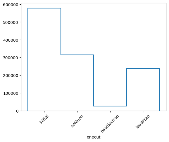
The histograms are now by default weighted, but like the print function this can be explicitly toggled between using weighted=True|False.There’s no option to scale the histograms by a scalar, this is left to a user to do so afterwards.
whonecut, whcutflow, wlabels = wgtcutflow.yieldhist()
whonecut.plot1d(yerr=0)
plt.xticks(plt.gca().get_xticks(), wlabels, rotation=45)
plt.show()
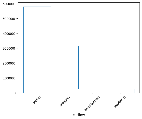
whcutflow.plot1d(yerr=0)
plt.xticks(plt.gca().get_xticks(), wlabels, rotation=45)
plt.show()
Saving to npz will include the weighted summary statistics by default, as well as a commonmask, but the actual weights (with the appropriate weightsmodifier) can also be saved directly, for later inspection.
npz = wgtcutflow.to_npz("cutflow_results_weighted.npz", includeweights=True)
print(npz)
npz.compute()
CutflowToNpz(file=cutflow_results_weighted.npz), labels=['initial', 'noMuon', 'twoElectron', 'leadPt20'], commonmasked=False, weighted=True, weightsmodifier=None)
with np.load("cutflow_results_weighted.npz") as f2:
    for i in f2.files:
        print(f"{i}: {f2[i]}")
labels: ['initial' 'noMuon' 'twoElectron' 'leadPt20']
nevonecut: [40 28  5 17]
nevcutflow: [40 28  5  3]
masksonecut: [[ True  True  True  True False False False  True  True  True False  True
   True  True False  True  True  True  True  True  True  True  True False
  False  True False  True False  True False False  True  True False  True
   True  True  True  True]
 [False False  True  True False False False False False False False False
  False False False False False False  True False  True  True False False
  False False False False False False False False False False False False
  False False False False]
 [False  True  True False  True  True  True False False  True False False
  False False False  True  True False False False  True  True False  True
   True False  True  True False  True False  True False  True False False
  False False False False]]
maskscutflow: [[ True  True  True  True False False False  True  True  True False  True
   True  True False  True  True  True  True  True  True  True  True False
  False  True False  True False  True False False  True  True False  True
   True  True  True  True]
 [False False  True  True False False False False False False False False
  False False False False False False  True False  True  True False False
  False False False False False False False False False False False False
  False False False False]
 [False False  True False False False False False False False False False
  False False False False False False False False  True  True False False
  False False False False False False False False False False False False
  False False False False]]
wgtevonecut: [578762.43554688 315450.42382812  25807.2109375  237244.12109375]
wgtevcutflow: [578762.43554688 315450.42382812  25807.2109375   26331.20117188]
weights: [ 26331.20117188  26331.20117188  26331.20117188  25807.2109375
  26331.20117188  26331.20117188 -26331.20117188  26067.890625
  26331.20117188  26331.20117188  26331.20117188  26331.20117188
  26331.20117188 -26331.20117188  26331.20117188  26331.20117188
 -26067.890625    26331.20117188 -26331.20117188  26331.20117188
  26331.20117188 -26331.20117188  26331.20117188  26331.20117188
  26331.20117188  26331.20117188  26331.20117188  26331.20117188
  26331.20117188  26331.20117188  26331.20117188  26331.20117188
  26331.20117188 -26331.20117188  26331.20117188 -26331.20117188
  26331.20117188 -26331.20117188  26331.20117188 -26331.20117188]
Commonmask support in cutflows / nminusones#
The commonmask feature allows one to specify a boolean array that is applied to every individual and combination of cuts, as well as the initial counts. Orthogonal selections like a cut for channels or gen-level requirements can be specified independant of cuts applied to all channels, e.g. cuts on jet multiplicity or invariant masses, while allowing studies in individual ‘channels.’ This serves two purposes, one permitting the same studies with fewer masks in the PackedSelection (which in a very complex analysis might not fit into the widest storage backend) or even injecting ‘external’ boolean arrays, and two, allowing the single cuts and cutflows to be interpreted from more complex initial states than all events in a sample.
selection.add_multiple(
    {
        "lheTaus": ak.sum(np.abs(events.LHEPart.pdgId) == 15, axis=1) >= 2,
        "lheMuons": ak.sum(np.abs(events.LHEPart.pdgId) == 13, axis=1) >= 2,
        "lheElectrons": ak.sum(np.abs(events.LHEPart.pdgId) == 11, axis=1) >= 2,
    }
)
taucutflow = selection.cutflow("noMuon", "twoElectron", "leadPt20", commonmask=selection.require(lheTaus=True))
elecutflow = selection.cutflow("noMuon", "twoElectron", "leadPt20", commonmask=selection.require(lheElectrons=True))
print("TAUS")
taucutflow.print()
print("ELECTRONS")
elecutflow.print()
TAUS
Cutflow selection stats:
Cut noMuon              :pass = 12                  cumulative pass = 12                  all = 18
-- eff = 66.7 %                    -- cumulative eff = 66.7 %
Cut twoElectron         :pass = 2                   cumulative pass = 2                   all = 18
-- eff = 11.1 %                    -- cumulative eff = 11.1 %
Cut leadPt20            :pass = 3                   cumulative pass = 0                   all = 18
-- eff = 16.7 %                    -- cumulative eff = 0.0 %
ELECTRONS
Cutflow selection stats:
Cut noMuon              :pass = 13                  cumulative pass = 13                  all = 13
-- eff = 100.0 %                    -- cumulative eff = 100.0 %
Cut twoElectron         :pass = 3                   cumulative pass = 3                   all = 13
-- eff = 23.1 %                    -- cumulative eff = 23.1 %
Cut leadPt20            :pass = 9                   cumulative pass = 3                   all = 13
-- eff = 69.2 %                    -- cumulative eff = 23.1 %
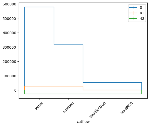
Categorical Axis fill for yieldhist and plot_vars#
In order to support subdividing a sample into subsamples or different channels in an efficient manner, a complex input categorical is available. This is expected to be a dictionary with several key-value pairs: axis: a hist.axis type including the axis features desired; values: an event-by-event array of fill values that should be passed into the histogram fill, and labels: the human-readable bin labels matching the axis passed in.
import hist

cwhonecut, cwhcutflow, cutlabels, catlabels = wgtcutflow.yieldhist(
    categorical={"axis": hist.axis.IntCategory([0, 41, 43], name="ttbarID"), "values": events.genTtbarId, "labels": ["X+jj", "X+c", "X+cc"]}
)

cwhcutflow.plot1d(yerr=0, overlay="ttbarID")
plt.xticks(plt.gca().get_xticks(), wlabels, rotation=45)
plt.legend()
plt.show()
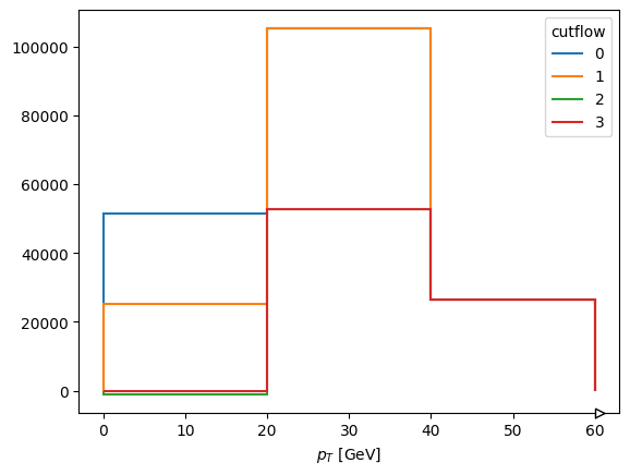
wch1, wch2, wclabels, catlabels = wgtcutflow.plot_vars(
    {"ept": events.Electron.pt, "ephi": events.Electron.phi},
    axes=[hist.axis.Regular(3, 0, 60, name="ept", label=r"$p_{T}$ [GeV]"), hist.axis.Regular(10, -3.14, 3.14, name="ephi", label=r"$\phi", circular=True)],
    categorical={"axis": hist.axis.IntCategory([0, 41, 43], name="ttbarID"), "values": events.genTtbarId, "labels": ["X+jj", "X+c", "X+cc"]},
)
wch2[0][:, :, 0].project("ept", "cutflow").plot1d(overlay="cutflow", yerr=False)
[StairsArtists(stairs=<matplotlib.patches.StepPatch object at 0x1450af750>, errorbar=None, legend_artist=None),
 StairsArtists(stairs=<matplotlib.patches.StepPatch object at 0x1450afed0>, errorbar=None, legend_artist=None),
 StairsArtists(stairs=<matplotlib.patches.StepPatch object at 0x145218050>, errorbar=None, legend_artist=None),
 StairsArtists(stairs=<matplotlib.patches.StepPatch object at 0x145218190>, errorbar=None, legend_artist=None)]
In CalVer coffea with mode="dask", everything happens in a delayed fashion. Therefore, PackedSelection can also operate in “dask” and fully support dask_awkward arrays. Use is still the same, but everything now is
a delayed dask type object which can be computed whenever the user wants to. This can be done by either calling .compute() on the object or dask.compute(*things).
PackedSelection can be initialized to operate in “dask” mode by instantiating with None and adding a dask_awkward array for the first time instead of an “eager” or “virtual” numpy or awkward array.
It should be noted that we only support dask_awkward arrays and not dask.array arrays. Please convert your dask arrays to dask_awkward via dask_awkward.from_dask_array(array). It is also not possible to mix materialized and delayed arrays in the same PackedSelection. Let’s now read the same events using dask and perform the exact same things.
import dask
import dask_awkward as dak

fname = "coffea/tests/samples/nano_dy.root"
dakevents = NanoEventsFactory.from_root(
    {fname: "Events"},
    metadata={"dataset": "nano_dy"},
    schemaclass=NanoAODSchema,
    mode="dask",
).events()

dakevents
dask.awkward<from-uproot, type='## * NanoEvents', npartitions=1>
Now dakevents is a delayed dask_awkward version of our events and if we compute it we get our normal events.
dakevents.compute()
[{Electron: [], PuppiMET: {phi: 1.64, ...}, FsrPhoton: [], ChsMET: {...}, ...},
 {Electron: [{deltaEtaSC: -0.0145, ...}], PuppiMET: {...}, FsrPhoton: [], ...},
 {Electron: [Electron, ...], PuppiMET: {...}, ...},
 {Electron: [Electron, ...], PuppiMET: {...}, ...},
 {Electron: [], PuppiMET: {phi: 0.538, ...}, FsrPhoton: [], ChsMET: {...}, ...},
 {Electron: [{deltaEtaSC: -0.0232, ...}], PuppiMET: {...}, FsrPhoton: [], ...},
 {Electron: [{deltaEtaSC: 0.00415, ...}], PuppiMET: {...}, FsrPhoton: [], ...},
 {Electron: [], PuppiMET: {phi: 0.105, ...}, FsrPhoton: [], ChsMET: {...}, ...},
 {Electron: [], PuppiMET: {phi: -0.513, ...}, FsrPhoton: [], ChsMET: ..., ...},
 {Electron: [{deltaEtaSC: 0.00813, ...}], PuppiMET: {...}, FsrPhoton: [], ...},
 ...,
 {Electron: [{deltaEtaSC: -0.00836, ...}], PuppiMET: {...}, ...},
 {Electron: [], PuppiMET: {phi: 0.612, ...}, FsrPhoton: [], ChsMET: {...}, ...},
 {Electron: [{deltaEtaSC: -0.00405, ...}], PuppiMET: {...}, ...},
 {Electron: [], PuppiMET: {phi: 2.83, ...}, FsrPhoton: [], ChsMET: {...}, ...},
 {Electron: [{deltaEtaSC: 0.053, ...}], PuppiMET: {...}, FsrPhoton: [], ...},
 {Electron: [], PuppiMET: {phi: 1.44, ...}, FsrPhoton: [], ChsMET: {...}, ...},
 {Electron: [{deltaEtaSC: -0.00986, ...}], PuppiMET: {...}, ...},
 {Electron: [], PuppiMET: {phi: -2.92, ...}, FsrPhoton: [], ChsMET: {...}, ...},
 {Electron: [], PuppiMET: {phi: -0.415, ...}, FsrPhoton: [], ChsMET: ..., ...}]
--------------------------------------------------------------------------------
backend: cpu
nbytes: 243.3 kB
type: 40 * event
Now we have to use dask_awkward instead of awkward and dakevents instead of events to do the same things. Let’s add the same (now delayed) arrays to PackedSelection.
selection = PackedSelection()

selection.add_multiple(
    {
        "twoElectron": dak.num(dakevents.Electron) == 2,
        "eleOppSign": dak.sum(dakevents.Electron.charge, axis=1) == 0,
        "noElectron": dak.num(dakevents.Electron) == 0,
        "twoMuon": dak.num(dakevents.Muon) == 2,
        "muOppSign": dak.sum(dakevents.Muon.charge, axis=1) == 0,
        "noMuon": dak.num(dakevents.Muon) == 0,
        "leadPt20": dak.any(dakevents.Electron.pt >= 20.0, axis=1) | dak.any(dakevents.Muon.pt >= 20.0, axis=1),
    }
)

print(selection)
PackedSelection(selections=('twoElectron', 'eleOppSign', 'noElectron', 'twoMuon', 'muOppSign', 'noMuon', 'leadPt20'), delayed_mode=True, items=7, maxitems=32)
Now, the same functions will return dask_awkward objects that have to be computed.
selection.all("twoElectron", "noMuon", "leadPt20")
dask.awkward<equal, type='## * bool', npartitions=1>
When computing those arrays we should get the same arrays that we got when operating in eager mode.
print(selection.all("twoElectron", "noMuon", "leadPt20").compute())
print(selection.require(twoElectron=True, noMuon=True, eleOppSign=False).compute())
[False, False, True, False, False, ..., False, False, False, False, False]
[False, False, False, True, False, ..., False, False, False, False, False]
Now, N-1 and cutflow will just return only delayed objects that must be computed.
dask_weights = Weights(None)
dask_weights.add("genweight", dakevents.genWeight)
nminusone = selection.nminusone("twoElectron", "noMuon", "leadPt20", weights=dask_weights, weightsmodifier=None)
nminusone
NminusOne(selections=('twoElectron', 'noMuon', 'leadPt20'), commonmasked=False, weighted=True, weightsmodifier=None)
It is again an NminusOne object which has the same methods.
Let’s look at the results of the N-1 selection in the same way
labels, nev, masks, _, wgtev, _, _ = nminusone.result()
labels, nev, masks, wgtev
(['initial', 'N - twoElectron', 'N - noMuon', 'N - leadPt20', 'N'],
 [dask.awkward<count, type=Scalar, dtype=int64>,
  dask.awkward<sum, type=Scalar, dtype=int64>,
  dask.awkward<sum, type=Scalar, dtype=int64>,
  dask.awkward<sum, type=Scalar, dtype=int64>,
  dask.awkward<sum, type=Scalar, dtype=int64>],
 [dask.awkward<equal, type='## * bool', npartitions=1>,
  dask.awkward<equal, type='## * bool', npartitions=1>,
  dask.awkward<equal, type='## * bool', npartitions=1>,
  dask.awkward<equal, type='## * bool', npartitions=1>],
 [dask.awkward<sum, type=Scalar, dtype=float32>,
  dask.awkward<sum, type=Scalar, dtype=float32>,
  dask.awkward<sum, type=Scalar, dtype=float32>,
  dask.awkward<sum, type=Scalar, dtype=float32>,
  dask.awkward<sum, type=Scalar, dtype=float32>])
Now however, you can see that everything is a dask awkward object (apart from the labels of course). If we compute them we should get the same things as before and indeed we do:
dask.compute(*nev), dask.compute(*masks), dask.compute(*wgtev)
((np.int64(40), np.int64(10), np.int64(3), np.int64(5), np.int64(3)),
 (<Array [False, True, True, False, ..., False, False, False] type='40 * bool'>,
  <Array [False, False, True, False, ..., False, False, False] type='40 * bool'>,
  <Array [False, False, True, True, ..., False, False, False] type='40 * bool'>,
  <Array [False, False, True, False, ..., False, False, False] type='40 * bool'>),
 (np.float32(578762.44),
  np.float32(105588.11),
  np.float32(26331.201),
  np.float32(25807.213),
  np.float32(26331.201)))
We can again print the statistics, however for this to happen, the object must of course compute the delayed nev list.
nminusone.print(weighted=True)
/Users/iason/Dropbox/work/pyhep_dev/coffea/src/coffea/analysis_tools.py:1062: UserWarning: Printing the N-1 selection statistics is going to compute dask_awkward objects.
  warnings.warn(
N-1 selection stats: (weighted)
Ignoring twoElectron pass = 105588.109375 all = 578762.4375 -- eff = 18.2 %
Ignoring noMuon pass = 26331.201171875 all = 578762.4375 -- eff = 4.5 %
Ignoring leadPt20 pass = 25807.212890625 all = 578762.4375 -- eff = 4.5 %
All cuts pass = 26331.201171875 all = 578762.4375 -- eff = 4.5 %
And now if we call result() again, the nev list is materialized.
nminusone.result().nev
[np.int64(40), np.int64(10), np.int64(3), np.int64(5), np.int64(3)]
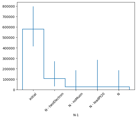
Again the histogram of your total event yields works. This time it is returns a hist.dask.Hist object.
h, labels = nminusone.yieldhist()
h
Weight() Σ=WeightedSum(value=0, variance=0)
It appears empty because it hasn’t been computed yet. Let’s do that.
h.compute()
Weight() Σ=WeightedSum(value=762820, variance=4.21972e+10)
Notice that this doesn’t happen in place as h is still not computed.
h
Weight() Σ=WeightedSum(value=0, variance=0)
We can again plot this histogram but we have to call plot on the computed one, otherwise it will just be empty.
h.compute().plot1d()
plt.xticks(plt.gca().get_xticks(), labels, rotation=45)
plt.show()
And we got exactly the same thing. Saving to .npz files is still possible but the delayed arrays will be naturally materalized while saving.
nminusone.to_npz("nminusone_results.npz")

with np.load("nminusone_results.npz") as f:
    for i in f.files:
        print(f"{i}: {f[i]}")
labels: ['initial' 'N - twoElectron' 'N - noMuon' 'N - leadPt20' 'N']
nev: [40 10  3  5  3]
masks: [[False  True  True False False False False False False  True False False
  False False False  True  True False False False  True  True False False
  False False False  True False  True False False False  True False False
  False False False False]
 [False False  True False False False False False False False False False
  False False False False False False False False  True  True False False
  False False False False False False False False False False False False
  False False False False]
 [False False  True  True False False False False False False False False
  False False False False False False  True False  True  True False False
  False False False False False False False False False False False False
  False False False False]
 [False False  True False False False False False False False False False
  False False False False False False False False  True  True False False
  False False False False False False False False False False False False
  False False False False]]
Same logic applies to the plot_vars function. Remember to use dakevents now and not events.
dask_categorical = {"axis": hist.axis.IntCategory([0, 41, 43], name="ttbarID"), "values": dakevents.genTtbarId, "labels": ["X+jj", "X+c", "X+cc"]}
hs, labels, catlabels = nminusone.plot_vars({"Ept": dakevents.Electron.pt, "Ephi": dakevents.Electron.phi}, categorical=dask_categorical)
hs[0].compute()[{"ttbarID": 0}].plot2d_full()
(ColormeshArtists(pcolormesh=<matplotlib.collections.QuadMesh object at 0x1483f0a50>, cbar=None, text=[]),
 [StairsArtists(stairs=<matplotlib.patches.StepPatch object at 0x1483f2ad0>, errorbar=<ErrorbarContainer object of 3 artists>, legend_artist=<ErrorbarContainer object of 3 artists>)],
 [StairsArtists(stairs=<matplotlib.patches.StepPatch object at 0x1483f3250>, errorbar=<ErrorbarContainer object of 3 artists>, legend_artist=<ErrorbarContainer object of 3 artists>)])
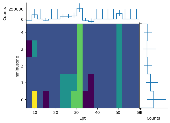
Those histograms are also delayed and have to be computed before plotting them.
Exactly the same things apply to the cutflow in delayed mode.