
Applying corrections to columnar data#
This is a rendered copy of applying_corrections.ipynb. You can optionally run it interactively on binder at this link
Here we will show how to apply corrections to columnar data using:
the
coffea.lookup_toolspackage, which was designed to read in ROOT histograms and a variety of data file formats popular within CMS into a standardized lookup table format;CMS-specific extensions to the above, for jet corrections (
coffea.jetmet_tools) and b-tagging efficiencies/uncertainties (coffea.btag_tools); while some subtools have been deprecated in favor of correctionlib, you may still come across older formats until everyone has fully transitioned.the correctionlib package, which provides an experiment-agnostic serializable data format for common correction functions. This format is the preferred format moving forward, as CMS has standardized on this.
Test data: We’ll use NanoEvents to construct some test data.
import awkward as ak
from coffea.nanoevents import NanoEventsFactory, NanoAODSchema

NanoAODSchema.warn_missing_crossrefs = False

fname = "coffea/tests/samples/nano_dy.root"
access_log = []
events = NanoEventsFactory.from_root(
    {fname: "Events"},
    schemaclass=NanoAODSchema,
    metadata={"dataset": "DYJets"},
    mode="virtual",
    access_log=access_log,
).events()
Coffea lookup_tools#
The entrypoint for coffea.lookup_tools is the extractor class.
from coffea.lookup_tools import extractor
%%bash
# download some sample correction sources
mkdir -p data
pushd data
PREFIX=https://raw.githubusercontent.com/scikit-hep/coffea/master/tests/samples
curl -Os $PREFIX/testSF2d.histo.root
curl -Os $PREFIX/Fall17_17Nov2017_V32_MC_L2Relative_AK4PFPuppi.jec.txt
curl -Os $PREFIX/Fall17_17Nov2017_V32_MC_Uncertainty_AK4PFPuppi.junc.txt
curl -Os $PREFIX/DeepCSV_102XSF_V1.btag.csv.gz
popd
~/Dropbox/work/pyhep_dev/coffea/binder/data ~/Dropbox/work/pyhep_dev/coffea/binder
~/Dropbox/work/pyhep_dev/coffea/binder
Opening a root file and using it as a lookup table#
In tests/samples, there is an example file with a TH2F histogram named scalefactors_Tight_Electron. The following code reads that histogram into an evaluator instance, under the key testSF2d and applies it to some electrons.
ext = extractor()
# several histograms can be imported at once using wildcards (*)
ext.add_weight_sets(["testSF2d scalefactors_Tight_Electron data/testSF2d.histo.root"])
ext.finalize()

evaluator = ext.make_evaluator()

print("available evaluator keys:")
for key in evaluator.keys():
    print("\t", key)
print("testSF2d:", evaluator["testSF2d"])
print("type of testSF2d:", type(evaluator["testSF2d"]))
available evaluator keys:
	 testSF2d
testSF2d: <coffea.lookup_tools.dense_lookup.dense_lookup object at 0x14c66c590> 2 dimensional histogram with axes:
	1: [-2.5   -2.    -1.566 -1.444 -0.8    0.     0.8    1.444  1.566  2.
  2.5  ]
	2: [ 10.  20.  35.  50.  90. 150. 500.]

type of testSF2d: <class 'coffea.lookup_tools.dense_lookup.dense_lookup'>
print("Electron eta:", events.Electron.eta)
print("Electron pt:", events.Electron.pt)
print("Scale factor:", evaluator["testSF2d"](events.Electron.eta, events.Electron.pt))
Electron eta: [??, ??, ??, ??, ??, ??, ??, ??, ??, ..., ??, ??, ??, ??, ??, ??, ??, ??, ??]
Electron pt: [??, ??, ??, ??, ??, ??, ??, ??, ??, ..., ??, ??, ??, ??, ??, ??, ??, ??, ??]
Scale factor: [[], [0.909], [0.953, 0.972], [0.807, 0.827], [], ..., [], [0.946], [], []]
Building and using your own correction from a histogram#
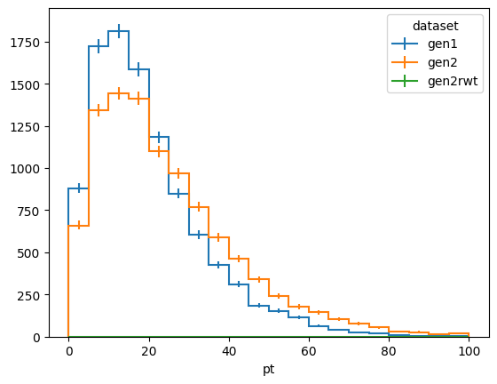
To use a histogram or ratio of histograms to build your own correction, you can use lookup_tools to simplify the implementation. Here we create some mock data for two slightly different pt and eta spectra (say, from two different generators) and derive a correction to reweight one sample to the other.
import numpy as np
import hist
import matplotlib.pyplot as plt

dists = (
    hist.Hist.new.StrCat(["gen1", "gen2", "gen2rwt"], name="dataset")
    .Reg(20, 0, 100, name="pt")
    .Reg(4, -3, 3, name="eta")
    .Weight()
    .fill(
        dataset="gen1",
        pt=np.random.exponential(scale=10.0, size=10000) + np.random.exponential(scale=10.0, size=10000),
        eta=np.random.normal(scale=1, size=10000),
    )
    .fill(
        dataset="gen2",
        pt=np.random.exponential(scale=10.0, size=10000) + np.random.exponential(scale=15.0, size=10000),
        eta=np.random.normal(scale=1.1, size=10000),
    )
)

fig, ax = plt.subplots()
dists[:, :, sum].plot1d(ax=ax)
ax.legend(title="dataset")
/Users/iason/micromamba/envs/awkward-coffea/lib/python3.13/site-packages/mplhep/utils.py:652: RuntimeWarning: All sumw are zero!  Cannot compute meaningful error bars
  return np.abs(method_fcn(self.values(), variances) - self.values())
<matplotlib.legend.Legend at 0x156eb2e90>
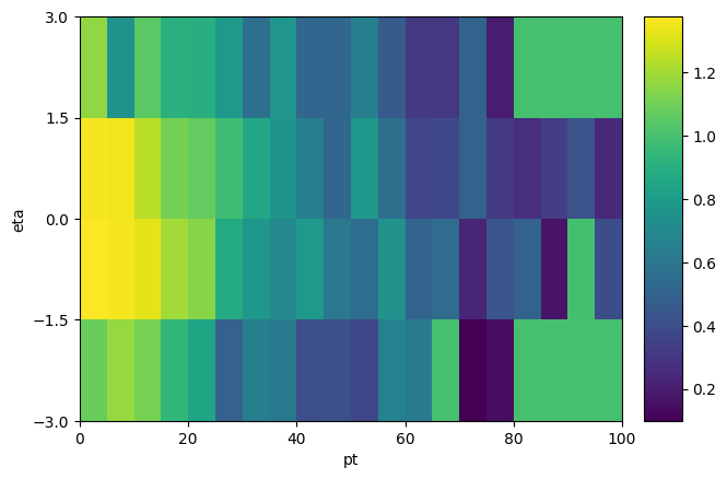
Now we derive a correction as a function of $p_T$ and $\eta$ to gen2 such that it agrees with gen1. We’ll set it to 1 anywhere we run out of statistics for the correction, to avoid divide by zero issues
from coffea.lookup_tools.dense_lookup import dense_lookup

num = dists["gen1", :, :].values()
den = dists["gen2", :, :].values()
sf = np.where(
    (num > 0) & (den > 0),
    num / np.maximum(den, 1) * den.sum() / num.sum(),
    1.0,
)

corr = dense_lookup(sf, [ax.edges for ax in dists.axes[1:]])
print(corr)

# a quick way to plot the scale factor is to steal the axis definitions from the input histograms:
sfhist = hist.Hist(*dists.axes[1:], data=sf)
sfhist.plot2d()
<coffea.lookup_tools.dense_lookup.dense_lookup object at 0x156f1d310> 2 dimensional histogram with axes:
	1: [  0.   5.  10.  15.  20.  25.  30.  35.  40.  45.  50.  55.  60.  65.
  70.  75.  80.  85.  90.  95. 100.]
	2: [-3.  -1.5  0.   1.5  3. ]
ColormeshArtists(pcolormesh=<matplotlib.collections.QuadMesh object at 0x156dd7a10>, cbar=<matplotlib.colorbar.Colorbar object at 0x156eb5160>, text=[])
Now we generate some new mock data as if it was drawn from gen2 and reweight it with our corr to match gen1
ptvals = np.random.exponential(scale=10.0, size=10000) + np.random.exponential(scale=15.0, size=10000)
etavals = np.random.normal(scale=1.1, size=10000)

dists.fill(dataset="gen2rwt", pt=ptvals, eta=etavals, weight=corr(ptvals, etavals))

fig, ax = plt.subplots()
dists[:, :, sum].plot1d(ax=ax)
ax.legend(title="dataset")
<matplotlib.legend.Legend at 0x1570c2990>
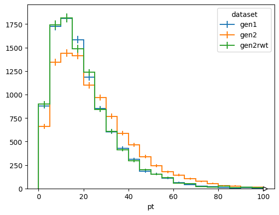
Note that corr() can accept also jagged arrays if need be.
CMS high-level tools#
Applying energy scale transformations with jetmet_tools#
The coffea.jetmet_tools package provides a convenience class CorrectedJetsFactory which applies specified corrections and computes uncertainties in one call. First we build the desired jet correction stack to apply. This will usually be some set of the various JEC and JER correction text files that depends on the jet cone size (AK4, AK8) and the pileup mitigation algorithm, as well as the data-taking year they are associated with.
from coffea.jetmet_tools import FactorizedJetCorrector, JetCorrectionUncertainty
from coffea.jetmet_tools import JECStack, CorrectedJetsFactory
import numpy as np

ext = extractor()
ext.add_weight_sets(
    [
        "* * data/Fall17_17Nov2017_V32_MC_L2Relative_AK4PFPuppi.jec.txt",
        "* * data/Fall17_17Nov2017_V32_MC_Uncertainty_AK4PFPuppi.junc.txt",
    ]
)
ext.finalize()

jec_stack_names = ["Fall17_17Nov2017_V32_MC_L2Relative_AK4PFPuppi", "Fall17_17Nov2017_V32_MC_Uncertainty_AK4PFPuppi"]

evaluator = ext.make_evaluator()

jec_inputs = {name: evaluator[name] for name in jec_stack_names}
jec_stack = JECStack(jec_inputs)
### more possibilities are available if you send in more pieces of the JEC stack
# mc2016_ak8_jxform = JECStack(["more", "names", "of", "JEC parts"])

print(dir(evaluator))
['Fall17_17Nov2017_V32_MC_L2Relative_AK4PFPuppi', 'Fall17_17Nov2017_V32_MC_Uncertainty_AK4PFPuppi']
Now we prepare some auxilary variables that are used to parameterize the jet energy corrections, such as jet area, mass, and event $\rho$ (mean pileup energy density), and pass all of these into the CorrectedJetsFactory:
name_map = jec_stack.blank_name_map
name_map["JetPt"] = "pt"
name_map["JetMass"] = "mass"
name_map["JetEta"] = "eta"
name_map["JetA"] = "area"

jets = events.Jet

jets["pt_raw"] = (1 - jets["rawFactor"]) * jets["pt"]
jets["mass_raw"] = (1 - jets["rawFactor"]) * jets["mass"]
jets["pt_gen"] = ak.values_astype(ak.fill_none(jets.matched_gen.pt, 0), np.float32)
jets["Rho"] = ak.broadcast_arrays(events.fixedGridRhoFastjetAll, jets.pt)[0]
name_map["ptGenJet"] = "pt_gen"
name_map["ptRaw"] = "pt_raw"
name_map["massRaw"] = "mass_raw"
name_map["Rho"] = "Rho"

corrector = FactorizedJetCorrector(
    Fall17_17Nov2017_V32_MC_L2Relative_AK4PFPuppi=evaluator["Fall17_17Nov2017_V32_MC_L2Relative_AK4PFPuppi"],
)
uncertainties = JetCorrectionUncertainty(Fall17_17Nov2017_V32_MC_Uncertainty_AK4PFPuppi=evaluator["Fall17_17Nov2017_V32_MC_Uncertainty_AK4PFPuppi"])

jet_factory = CorrectedJetsFactory(name_map, jec_stack)
corrected_jets = jet_factory.build(jets)

print("starting columns:", set(ak.fields(jets)))
print("new columns:", set(ak.fields(corrected_jets)) - set(ak.fields(jets)))
starting columns: {'nConstituents', 'rawFactor', 'electronIdx2', 'nElectrons', 'btagDeepFlavC', 'Rho', 'pt_gen', 'chHEF', 'bRegCorr', 'btagDeepFlavB', 'partonFlavour', 'genJetIdxG', 'genJetIdx', 'muonIdx2', 'btagDeepC', 'electronIdxG', 'electronIdx1G', 'pt_raw', 'jercCHF', 'muonIdx1', 'electronIdx1', 'mass', 'cleanmask', 'electronIdx2G', 'neEmEF', 'qgl', 'area', 'muonIdx2G', 'pt', 'muonIdxG', 'chEmEF', 'bRegRes', 'btagDeepB', 'hadronFlavour', 'jetId', 'btagCSVV2', 'btagCMVA', 'muonSubtrFactor', 'mass_raw', 'phi', 'nMuons', 'muEF', 'jercCHPUF', 'neHEF', 'puId', 'eta', 'muonIdx1G'}
new columns: {'jet_energy_uncertainty_jes', 'pt_jec', 'pt_orig', 'JES_jes', 'jet_energy_correction', 'mass_jec', 'mass_orig'}
Below we show that the corrected jets indeed have a different $p_T$ and mass than we started with
print("untransformed pt ratios", jets.pt / jets.pt_raw)
print("untransformed mass ratios", jets.mass / jets.mass_raw)

print("transformed pt ratios", corrected_jets.pt / corrected_jets.pt_raw)
print("transformed mass ratios", corrected_jets.mass / corrected_jets.mass_raw)

print("JES UP pt ratio", corrected_jets.JES_jes.up.pt / corrected_jets.pt_raw)
print("JES DOWN pt ratio", corrected_jets.JES_jes.down.pt / corrected_jets.pt_raw)
untransformed pt ratios [[1.12, 1.09, 1.2, 1.35, 1.27], [1.03, 1.08, ..., 1, 0.918], ..., [1.13, 0.978]]
untransformed mass ratios [[1.12, 1.09, 1.2, 1.35, 1.27], [1.03, 1.08, ..., 1, 0.918], ..., [1.13, 0.978]]
transformed pt ratios [[1.2, 1.3, 1.46, 2.09, 2.1], [1.09, 1.29, ..., 1.22, 1.83], ..., [1.37, 1.15]]
transformed mass ratios [[1.2, 1.3, 1.46, 2.09, 2.1], [1.09, 1.29, ..., 1.22, 1.83], ..., [1.37, 1.15]]
JES UP pt ratio [[1.22, 1.35, 1.56, 2.34, 2.37], [1.1, 1.32, ..., 1.94], ..., [1.41, 1.17]]
JES DOWN pt ratio [[1.19, 1.25, 1.35, 1.83, 1.83], [1.08, 1.26, ..., 1.73], ..., [1.33, 1.12]]
Applying CMS b-tagging corrections with btag_tools#
The coffea.btag_tools module provides the high-level utility BTagScaleFactor which calculates per-jet weights for b-tagging as well as light flavor mis-tagging efficiencies. Uncertainties can be calculated as well.
from coffea.btag_tools import BTagScaleFactor

btag_sf = BTagScaleFactor("data/DeepCSV_102XSF_V1.btag.csv.gz", "medium")

print("SF:", btag_sf.eval("central", events.Jet.hadronFlavour, abs(events.Jet.eta), events.Jet.pt))
print("systematic +:", btag_sf.eval("up", events.Jet.hadronFlavour, abs(events.Jet.eta), events.Jet.pt))
print("systematic -:", btag_sf.eval("down", events.Jet.hadronFlavour, abs(events.Jet.eta), events.Jet.pt))
SF: [[1.52, 1.56, 1.59, 1.6, 1.6], [0.969, 1.57, ..., 1.6, 1.6], ..., [1.6, 1.6]]
systematic +: [[1.72, 1.77, 1.79, 1.8, 1.8], [1.01, 1.78, ..., 1.8, 1.8], ..., [1.8, 1.8]]
systematic -: [[1.31, 1.36, 1.38, 1.4, 1.4], [0.925, 1.37, ..., 1.4, 1.4], ..., [1.4, 1.4]]
Using correctionlib#
For the most part, using correctionlib is straightforward. We’ll show here how to convert the custom correction we derived earlier (corr) into a correctionlib object, and save it in the json format:
import correctionlib
import rich
import correctionlib.convert

# without a name, the resulting object will fail validation
sfhist.name = "gen2_to_gen1"
sfhist.label = "out"
clibcorr = correctionlib.convert.from_histogram(sfhist)
clibcorr.description = "Reweights gen2 to agree with gen1"
# set overflow bins behavior (default is to raise an error when out of bounds)
clibcorr.data.flow = "clamp"

cset = correctionlib.schemav2.CorrectionSet(
    schema_version=2,
    description="my custom corrections",
    corrections=[clibcorr],
)
rich.print(cset)

with open("data/mycorrections.json", "w") as fout:
    fout.write(cset.model_dump_json(exclude_unset=True))
CorrectionSet (schema v2)
my custom corrections
📂
└── 📈 gen2_to_gen1 (v0)
    Reweights gen2 to agree with gen1
    Node counts: MultiBinning: 1
    ╭──────────── ▶ input ─────────────╮ ╭──────────── ▶ input ────────────╮
    │ pt (real)                        │ │ eta (real)                      │
    │ pt                               │ │ eta                             │
    │ Range: [0.0, 100.0), overflow ok │ │ Range: [-3.0, 3.0), overflow ok │
    ╰──────────────────────────────────╯ ╰─────────────────────────────────╯
    ╭─── ◀ output ───╮
    │ out (real)     │
    │ No description │
    ╰────────────────╯
We can now use this new correction in a similar way to the original corr() object:
ceval = cset.to_evaluator()

ceval["gen2_to_gen1"].evaluate(ptvals, etavals)
array([1.34972203, 0.98072826, 1.34972203, ..., 1.20142093, 0.51586373,
       1.32139074], shape=(10000,))
def myJetSF(jets):
    # Older correctionlib did not handle jagged arrays\
    # the solution for flattening and unflattening is left commented below
    # j, nj = ak.flatten(jets), ak.num(jets)
    # sf = ceval["gen2_to_gen1"].evaluate(np.array(j.pt), np.array(j.eta))
    # return ak.unflatten(sf, nj)
    return ceval["gen2_to_gen1"].evaluate(jets.pt, jets.eta)


myJetSF(events.Jet)
[[1, 0.514, 0.787, 0.91, 0.91],
 [0.398, 0.765, 0.981, 0.941, 0.91, 0.941, 1.11, 0.91],
 [1, 0.505, 0.738, 0.646, 0.854],
 [0.621, 0.613, 0.941],
 [0.426, 0.271, 0.787, 0.941, 0.941],
 [0.698, 0.765, 0.774, 0.88, 0.906, 0.941, 0.91, 1.2],
 [1, 0.777, 0.613, 0.491],
 [0.613, 0.491, 0.906, 0.941],
 [0.906],
 [0.994, 0.609, 0.765, 0.774, 0.491, 0.787, 0.91, 1.11, 0.91],
 ...,
 [0.861, 0.88],
 [0.906, 0.91, 0.91, 0.91],
 [0.514, 0.523, 0.491, 1.14, 1.2, 0.941, 1.11, 1.11, 0.91],
 [0.791, 0.787, 0.88],
 [1.14, 1.2],
 [0.981, 0.854, 1.2],
 [1.07],
 [0.459, 0.646, 0.854, 0.906, 0.854, 1.2],
 [0.941, 1.11]]
--------------------------------------------------------------
backend: cpu
nbytes: 1.8 kB
type: 40 * var * float64
In dask mode, the only difference is that you need to call compute on stuff
fname = "coffea/tests/samples/nano_dy.root"
events = NanoEventsFactory.from_root(
    {fname: "Events"},
    schemaclass=NanoAODSchema,
    metadata={"dataset": "DYJets"},
    mode="dask",
).events()
name_map = jec_stack.blank_name_map
name_map["JetPt"] = "pt"
name_map["JetMass"] = "mass"
name_map["JetEta"] = "eta"
name_map["JetA"] = "area"

jets = events.Jet

jets["pt_raw"] = (1 - jets["rawFactor"]) * jets["pt"]
jets["mass_raw"] = (1 - jets["rawFactor"]) * jets["mass"]
jets["pt_gen"] = ak.values_astype(ak.fill_none(jets.matched_gen.pt, 0), np.float32)
jets["Rho"] = ak.broadcast_arrays(events.fixedGridRhoFastjetAll, jets.pt)[0]
name_map["ptGenJet"] = "pt_gen"
name_map["ptRaw"] = "pt_raw"
name_map["massRaw"] = "mass_raw"
name_map["Rho"] = "Rho"

corrector = FactorizedJetCorrector(
    Fall17_17Nov2017_V32_MC_L2Relative_AK4PFPuppi=evaluator["Fall17_17Nov2017_V32_MC_L2Relative_AK4PFPuppi"],
)
uncertainties = JetCorrectionUncertainty(Fall17_17Nov2017_V32_MC_Uncertainty_AK4PFPuppi=evaluator["Fall17_17Nov2017_V32_MC_Uncertainty_AK4PFPuppi"])

jet_factory = CorrectedJetsFactory(name_map, jec_stack)
corrected_jets = jet_factory.build(jets)

print("starting columns:", set(ak.fields(jets)))
print("new columns:", set(ak.fields(corrected_jets)) - set(ak.fields(jets)))
starting columns: {'nConstituents', 'rawFactor', 'electronIdx2', 'nElectrons', 'btagDeepFlavC', 'Rho', 'pt_gen', 'chHEF', 'bRegCorr', 'btagDeepFlavB', 'partonFlavour', 'genJetIdxG', 'genJetIdx', 'muonIdx2', 'btagDeepC', 'electronIdxG', 'electronIdx1G', 'pt_raw', 'jercCHF', 'muonIdx1', 'electronIdx1', 'mass', 'cleanmask', 'electronIdx2G', 'neEmEF', 'qgl', 'area', 'muonIdx2G', 'pt', 'muonIdxG', 'chEmEF', 'bRegRes', 'btagDeepB', 'hadronFlavour', 'jetId', 'btagCSVV2', 'btagCMVA', 'muonSubtrFactor', 'mass_raw', 'phi', 'nMuons', 'muEF', 'jercCHPUF', 'neHEF', 'puId', 'eta', 'muonIdx1G'}
new columns: {'jet_energy_uncertainty_jes', 'pt_jec', 'pt_orig', 'JES_jes', 'jet_energy_correction', 'mass_jec', 'mass_orig'}
print("untransformed pt ratios", (jets.pt / jets.pt_raw).compute())
print("untransformed mass ratios", (jets.mass / jets.mass_raw).compute())

print("transformed pt ratios", (corrected_jets.pt / corrected_jets.pt_raw).compute())
print("transformed mass ratios", (corrected_jets.mass / corrected_jets.mass_raw).compute())

print("JES UP pt ratio", (corrected_jets.JES_jes.up.pt / corrected_jets.pt_raw).compute())
print("JES DOWN pt ratio", (corrected_jets.JES_jes.down.pt / corrected_jets.pt_raw).compute())
untransformed pt ratios [[1.12, 1.09, 1.2, 1.35, 1.27], [1.03, 1.08, ..., 1, 0.918], ..., [1.13, 0.978]]
untransformed mass ratios [[1.12, 1.09, 1.2, 1.35, 1.27], [1.03, 1.08, ..., 1, 0.918], ..., [1.13, 0.978]]
transformed pt ratios [[1.2, 1.3, 1.46, 2.09, 2.1], [1.09, 1.29, ..., 1.22, 1.83], ..., [1.37, 1.15]]
transformed mass ratios [[1.2, 1.3, 1.46, 2.09, 2.1], [1.09, 1.29, ..., 1.22, 1.83], ..., [1.37, 1.15]]
JES UP pt ratio [[1.22, 1.35, 1.56, 2.34, 2.37], [1.1, 1.32, ..., 1.94], ..., [1.41, 1.17]]
JES DOWN pt ratio [[1.19, 1.25, 1.35, 1.83, 1.83], [1.08, 1.26, ..., 1.73], ..., [1.33, 1.12]]
myJetSF(events.Jet)
dask.awkward<gen2-to, type='## * var * float64', npartitions=1>
myJetSF(events.Jet).compute()
[[1, 0.514, 0.787, 0.91, 0.91],
 [0.398, 0.765, 0.981, 0.941, 0.91, 0.941, 1.11, 0.91],
 [1, 0.505, 0.738, 0.646, 0.854],
 [0.621, 0.613, 0.941],
 [0.426, 0.271, 0.787, 0.941, 0.941],
 [0.698, 0.765, 0.774, 0.88, 0.906, 0.941, 0.91, 1.2],
 [1, 0.777, 0.613, 0.491],
 [0.613, 0.491, 0.906, 0.941],
 [0.906],
 [0.994, 0.609, 0.765, 0.774, 0.491, 0.787, 0.91, 1.11, 0.91],
 ...,
 [0.861, 0.88],
 [0.906, 0.91, 0.91, 0.91],
 [0.514, 0.523, 0.491, 1.14, 1.2, 0.941, 1.11, 1.11, 0.91],
 [0.791, 0.787, 0.88],
 [1.14, 1.2],
 [0.981, 0.854, 1.2],
 [1.07],
 [0.459, 0.646, 0.854, 0.906, 0.854, 1.2],
 [0.941, 1.11]]
--------------------------------------------------------------
backend: cpu
nbytes: 1.8 kB
type: 40 * var * float64